Python to replace SAS Enterprise Miner (basic)
Why?
The last fall (2012) I took a class called Business Intelligence (at UT Dallas) which is the same as Data Mining or Machine Learning to business people. On that class they taught us to use SAS Enterprise Miner. I used it but I hate to use it. First of all I had to pay for it: like $100 dollars, not much because the University has an arrangement with SAS but I had to pay that again soon, and I have to pay a lot of money to use it without the University help. Second, is slow as hell, I was going mad using that piece of $%#^ :-P. And don’t get me wrong, the software is “good”, but is not for me.
That is the reason why during this time I learn the basics of R (from coursera) and python data analysis packages, mainly pandas. The objective on this case is to use Python to replace the functionality I learned this semester of SAS Enterprise Miner. I already knew basic the basics of pandas, numpy and scipy but I still had on my ToDo list learn Scikit-learn.
What I wanted to do
I wanted to replace the functionality I learned this semester from SAS EM, that is, the very basics:
- Import data
- Basic data transformation
- Model training
- Model comparison
- Model scoring
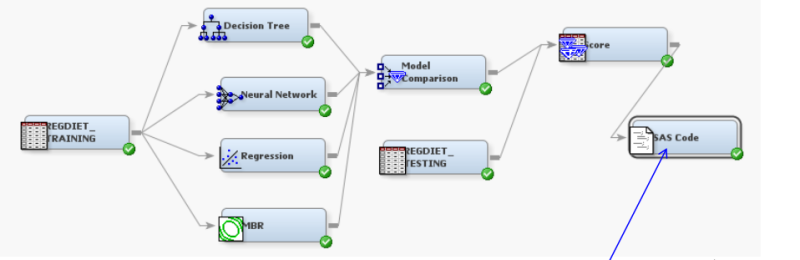
So I needed to do the same with iPython, Pandas, Scikit-learn and Matplotlib. On SAS EM a basic project looks like this:
Installation
I already had installed iPython, pandas and numpy but not Scikit-learn,
and since I am using Python 3 (3.2.3) I had to compile scikit-learn from
the last development source code: as easy as download the last version
from Github and ran python setup.py install
Example
The data I used is the same I used for a project on the Business Intelligence class, so I could compare the results I obtained from SAS.
In a tweet the project is: The data is from people who order products
from a catalog, and the idea was to help the company to target the
customers who receive the catalogs in order to reduce expenses. There
are two CSV files of 2000 records each, one for training and one for
testing. The available data is:
- NGIF: number of orders in the 24 months
- RAMN: Total order amounts in dollars in the last 24 months
- LASG: Amount of last order
- LASD: Date of last order (you may need to convert it to number of months elapsed to 01/01/2007)
- RFA1: Frequency of order
- 1=One order in the last 24 months
- 2=Two orders in the last 24 months
- 3=Three orders in the last 24 months
- 4=Four or more orders in the last 24 months
- RFA2: Order amount category (as defined by the firm) of the last
order
- 1=$0.01 - $1.99
- 2=$2.00 - $2.99
- 3=$3.00 e - $4.99
- 4=$5.00 - $9.99
- 5=$10.00 - $14.99
- 6=$15.00 - $24.99
- 7=$25.00 and above
- Money: money amount eventually a customer will spend on next order (if she places orders), only available for “testing”.
- Order: Actual response (1: response, 0: no response)
The file looks like this:
CustomerID,NGIF,RAMN,LASG,LASD,RFA1,RFA2,Order
1,2,30,20,200503,1,6,1
2,25,207,20,200503,1,6,0
3,5,52,15,200503,1,6,0
4,11,105,15,200503,1,6,0
5,2,32,17,200503,1,6,0
...
The good part is that the data is clean, everything is a number and there are no missing values. This is far from real, but for a first example is perfect.
1. Import data
As simple as:
train = pd.read_csv('training.csv')
test = pd.read_csv('testing.csv')
train = train.set_index('CustomerID')
test = test.set_index('CustomerID')
2. Data transform
Is necesary to convert the LASG (Date of last order) to a normal number;
I decide to use MSLO (number of Months Since Last Order). Knowing that
the data is from February, 2007 the equation to convert I use is:
MSLO = 12*(2007 - YEAR) - MONTH + 2. On python it translates to:
MSLO = train['LASD']
f = lambda x: 12 * (2007 - int(str(x)[0:4])) - int(str(x)[4:6]) + 2
MSLO = MSLO.apply(f)
Then just need to remove the LASD column and add the MSLO data:
del train['LASD']
train['MSLO'] = MSLO
3. Model Training
This is covered by scikit-learn, they have tons of models, from Decision Tree to a lot of models, seriously. For this example I use the always good Decision Tree also Support Vector Machine and Naive Bayes.
X_train = train[['NGIF', 'RAMN', 'LASG', 'MSLO', 'RFA1',
'RFA2']].values
Y_train = train['Order'].values

svm = SVC()
svm.probability = True
svm.fit(X_train, Y_train)

tree = DecisionTreeClassifier(max_depth=6)
tree.fit(X_train, Y_train)
out = export_graphviz(tree, out_file='tree.dot')

gnb = GaussianNB()
gnb.fit(X_train, Y_train)
4. Model Scoring/Comparison
Scikit-learn comes with Confusion Matrix and ROC Chart included:
tree_score = tree.predict(X_test)
svm_score = svm.predict(X_test)
gnb_score = gnb.predict(X_test)

tree_cm = confusion_matrix(Y_test, tree_score)
svm_cm = confusion_matrix(Y_test, svm_score)
gnb_cm = confusion_matrix(Y_test, gnb_score)
# tree
array([[1365, 67], [ 506, 62]])
# svm
array([[1362, 70], [ 531, 37]])
#gnb
array([[1196, 236], [ 406, 162]])tree_probas = tree.predict_proba(X_test)
svm_probas = svm.predict_proba(X_test)
gnb_probas = gnb.predict_proba(X_test)
tree_fpr, tree_tpr, tree_thresholds = roc_curve(Y_test,
tree_probas[:, 1])
svm_fpr, svm_tpr, svm_thresholds = roc_curve(Y_test,
svm_probas[:, 1])
gnb_fpr, gnb_tpr, gnb_thresholds = roc_curve(Y_test,
gnb_probas[:, 1])
pl.plot(tree_fpr, tree_tpr, label='Tree')
pl.plot(svm_fpr, svm_tpr, label='SVM')
pl.plot(gnb_fpr, gnb_tpr, label='GNB')
pl.xlabel('False Positive Rate')
pl.ylabel('True Positive Rate')
pl.title('Receiver operating characteristic')
pl.legend(loc="lower right")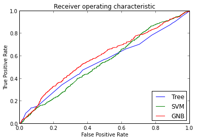
Conclusion
With this quick example I was able to get most of the results I learned on my BI class. The analysis of the results is more important but not the objective of this post. Enterprise Miner produces a lot of results but they are useless unless you understand them, is better to get few results and use understand them correctly. Other chart I learned was the Lift chart but scikit-learn does not have this option.
I was able to get the results a lot quicker with Python than with SAS EM, for this project it took me like 4 or 5 hours with SAS EM and less than 1 hour on Python.
The complete iPython notebook (also visible here) and data is available on Github: Data analysis Examples Python - Catalog Marketing.
Note : I know this is the most very basic example of Machine Learning on Python, more complex examples will come later.