Python Finance Package v0.035 - Event study and market simulator Integration
Ok, here come the first “Real Life” example. As I mention on previous posts my finance knowledge is mostly null so I cannot say this can be used on real life but what I found playing with the utils I have created is very interesting.
If anyone use this techniques and win/lose money I would love to hear :P Also if anyone find discrepancies on the results please tell me.
Changes since last time
- Bug Fixes on Multiple Event Study: Missing values are now filled: forward and then backwards.
- Multiple Event Studies: Graph with error bars (std)
- Integration between the Event Study Finder and Market Simulator
Example
- Use the S&P 500 symbols from 2012
- Look in all 2011 for events when the value of the stock went below $5
- Discover how to use this opportunity to invest on the equities
- Simulate if we would make some money from that
1. Setup
In [1]: Imports
import os
from datetime import datetime
from finance.utils import BasicUtils
from finance.utils import FileManager
from finance.utils import ListUtils
from finance.evtstudy import EventFinder
from finance.evtstudy import MultipleEvents
from finance.sim import MarketSimulator
In [2]: Download all the information on 2011 of all S&P 500 equities on 2012
SP500_2012 = ListUtils.SP500(year=2012)
fm = FileManager()
start = datetime(2011,1,1)
end = datetime(2011,12,31)
files = fm.get_data(SP500_2012, start, end)
len(files)
Out [2]:
4982. Event: Went Below 5 - One event per Equity
In [5]: Look for events
evtf = EventFinder()
evtf.symbols = SP500_2012
evtf.start_date = start
evtf.end_date = end
evtf.function = evtf.went_below(5)
evtf.search()
In [6]:
evtf.num_eventsOut [6]: 5 Events where found
5In [7]: Analyse the 5 Events
mevt = MultipleEvents()
mevt.list = evtf.list
mevt.market = 'SPY'
mevt.lookback_days = 20
mevt.lookforward_days = 20
mevt.estimation_period = 250
mevt.run()
In [8]: Graph the mean cumulative abnornal return
mevt.mean_cumulative_abnormal_return.plot()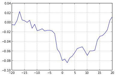
The graph tell us that in average after the event (day 0) the return goes up, but what about the risk?
In [9]: Print the Cumulative Abnormal Return with Error Bars
mevt.plot('car')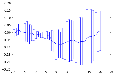 Mean CAR with
Ok, the graph tell us that the risk is going up as the time passes, this was expected. Since we are looking the data in 2011 we can see what happen in reality.
We use the market simulator but we create the orders from the event list. The instructions are:
- On the event day: Buy 100 shares
- 20 days after the event: Sell the 100 Shares
- Initial cash = $1000
In [10]: Use the market simulator
sim = MarketSimulator('./data')
sim.field = "Adj Close"
sim.initial_cash = 1000
sim.create_trades_from_event(evtf.list, eventDayAction='Buy',
eventDayShares=100, actionAfter='Sell', daysAfter=20, sharesAfter=100)
sim.simulate()
sim.trades
Out [10]: This are the trades generated by the Simulator
symbol action num_of_shares
2011-08-08 HBAN Buy 100
2011-09-06 HBAN Sell 100
2011-09-22 GNW Buy 100
2011-10-03 AMD Buy 100
2011-10-20 GNW Sell 100
2011-10-31 AMD Sell 100
2011-11-23 HCBK Buy 100
2011-12-19 BAC Buy 100
2011-12-22 HCBK Sell 100
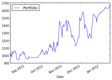
2012-01-19 BAC Sell 100In [11]: Graph of the portfolio value:
sim.portfolio.plot()
BasicUtils.total_return(sim.portfolio)
Out [11]:
0.501I obtain 5 events and a total return of 0.501 with just 10 trades.
3. Event: Went below 5 - more than one event per equity
From what I saw on the events when one event occurred more events occurred soon (less than 20 days later), that didn’t look good for me that’s why I tried first with no repeating events. But from my computational investing course I notice that they use all the events so I tried that to: The code is the same just change this on the event finder:
evtf.search(oneEventPerEquity=False)On this case I found 21 events with a total return of: 0.684; chart:
Conclusion
Also if anyone find discrepancies on the results please tell me.
First, I obtain a total return of 0.501 with just 10 trades; that means
that the final value of the portfolio was $1,501. When I saw this I was
amazed, just buying shares of very cheap stocks (100 stocks @ <$5 = 500) and then selling those stocks 20 days later was possible to make
$501 in just 6 months. Even more if use the second event study.
Second, the utils works very well together and with a considerable amount of data, not just 2 equities as before.
Third, I am rich! weee! Ok no, not really. But the results are very interesting, at least I was amazed, I never believe of finding a return greater than 0.5.
The code + the complete example is on GitHub: PythonFinance
This is far from the end but the computational investing course ends with this example so I have no longer a source of inspiration, I am searching for book on quantitative finance to keep learning and developing the package.